神经网络基本介绍

Neural network

Problems of too many features

If we wan to create a hypothesis consisting of all squares terms and cross terms, it will be an extremely complex function. For instance:

For computer vision, if we want to recognize a picture of 50 * 50px, there will be 2500 pixels. Then if we utilize every cross terms like $x_i \times x_j$ , there will be 300, 000 features.

origin of neural network

Algorithms that try to mimic the brain.

Very widely used in 80s and early 90s; popularity diminished in late 90s.

Resurgence(复兴): State-of-the-art(最高水平) technique for many application. Because neural network needs computational capacity, recent development and advancement of computer make it rise again

one learning algorithm hypothesis

Rewire other neuro to a certain part of brain. You can make the areas of the cerebral cortex that were listening to the sound see the image.

So maybe there’s a one learning algorithm that can process sight or sound or touch instead of needing to implement thousands of different programs.

Some amazing instances:

• Seeing with tongue. A system called BrainPort undergoing FDA trials.
• Human echolocation. Human sonar
• Haptic Belt 触觉腰带
• Transplat a third eye to a frog, it can learn to use it

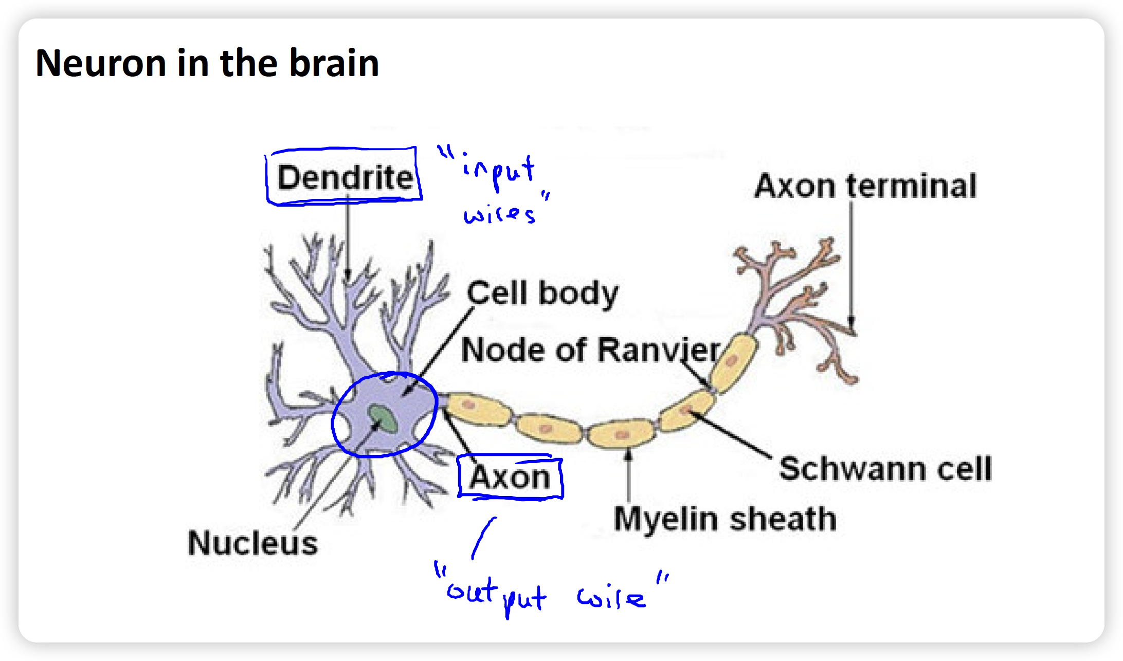
Dendrite树突: can be considered as input wires, which receive informations from other neurons.

Axon轴突: output. sends output via axon to other nodes.

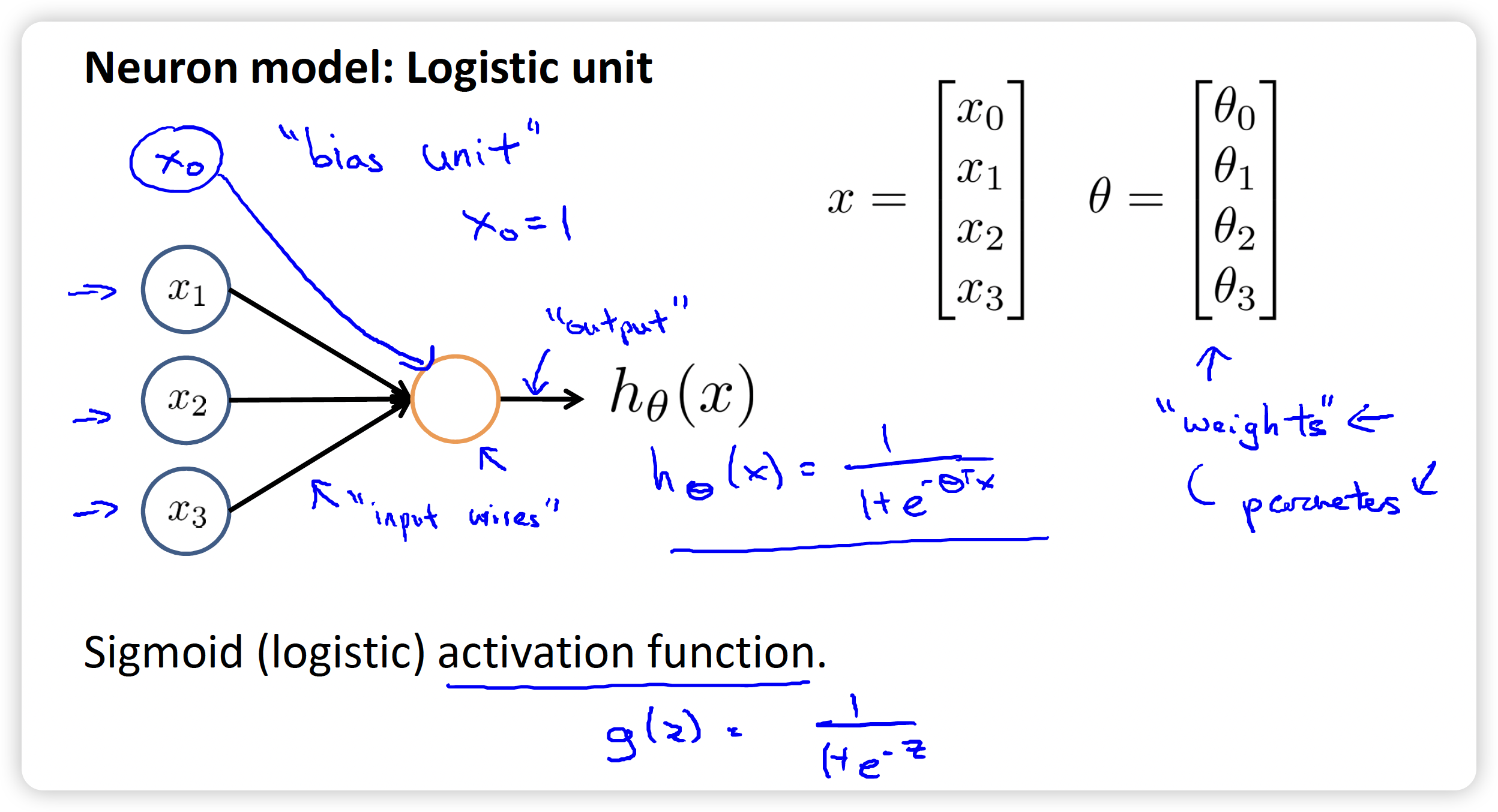
Like a neuron. Some features such as $x_1, x_2, x_3$are input to the neuron. Maybe also $x_0$, known as bias unit偏置单元, whose value is always 1. Then output to the hypothesis function $h_\theta (x)$

Some terminology:

• Sigmoid function may be called logistic activation function.
• Parameter $\theta$ may be called weights权重

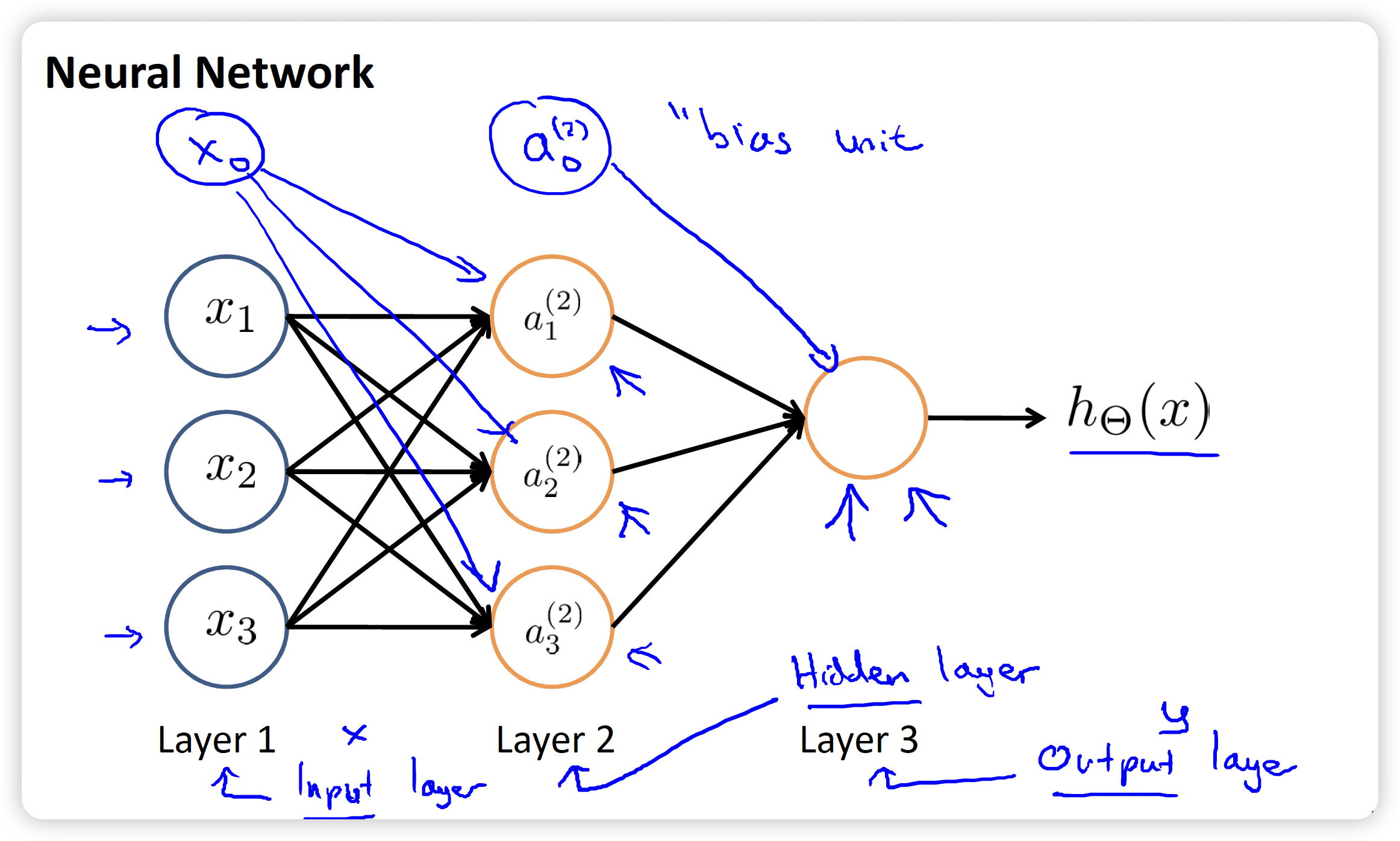
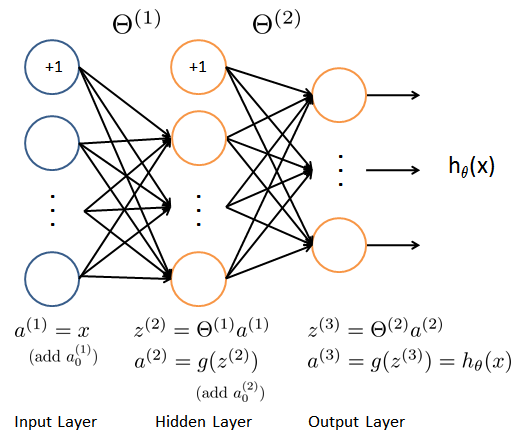
There are 3 features other than $x_0$ and 3 neurons $a_1, a_2, a_3$. The 3rd layer outputs the value that hypothesis function computes.

Three types of layer:

• Input layer. Features.
• Output layer.
• Between above two layers, is called hidden layer. Maybe more than 1 layer.

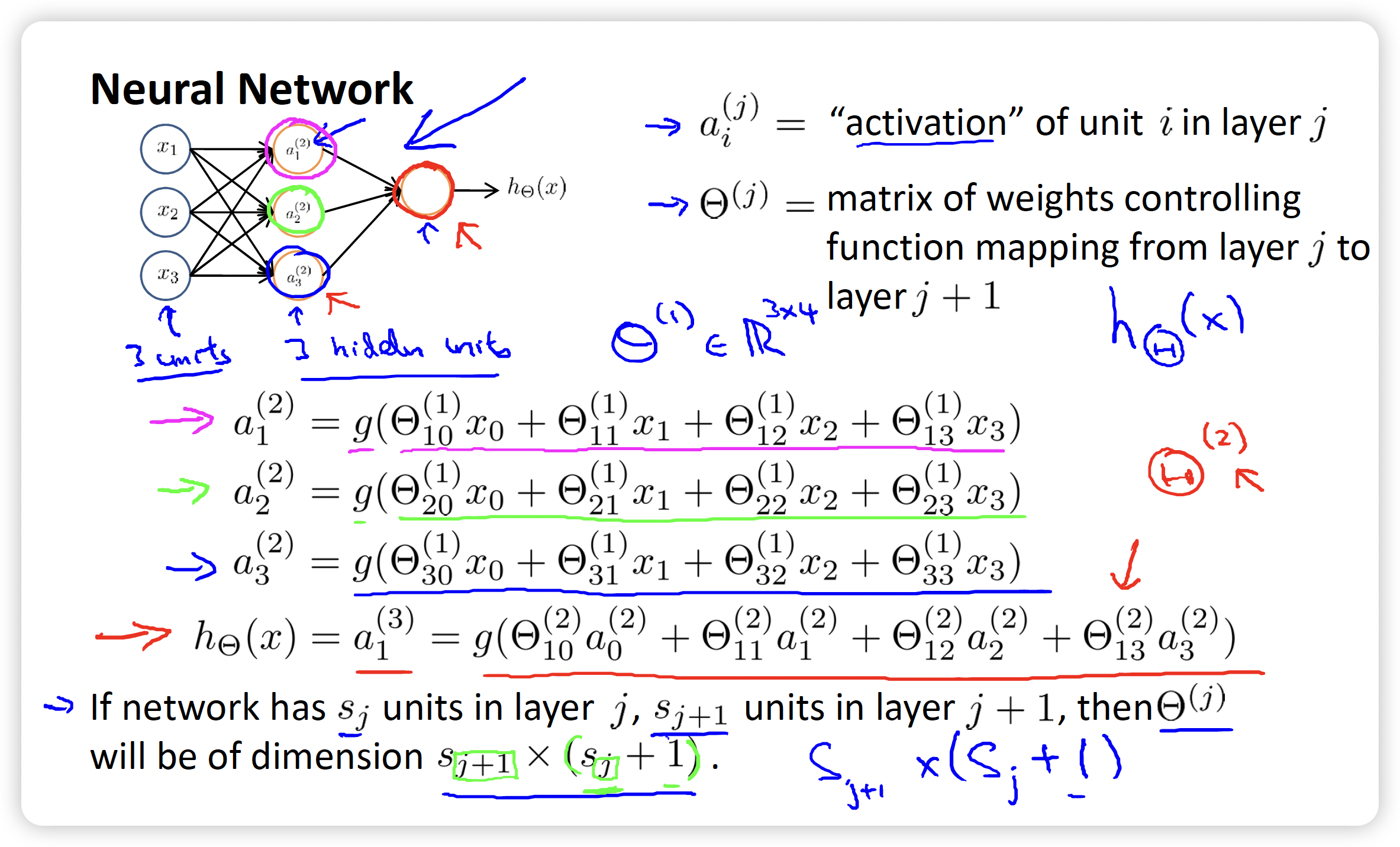
$\Theta$: The matrix of weights controlling function mapping form layer $j$ to layer $j + 1$.

Its dimension is determined by both $j$th layer and $j + 1$th layer:

• Row: equals the number of units in $j + 1$th layer
• Column: equals the number of units in $j$th layer + 1, because of the bias unit偏置单元

$a$: a unit.

Superscript indicates which layer it’s in; subscript indicates its position in its layer.

vectorization向量化

Create a matrix called $z$ to represent the product of $\Theta$ and $x$

$$\begin{align} z^{(2)} &= \Theta^{(1)} x = \Theta^{(1)} a^{(1)} \\ a^{(2)} &= g(z^{(2)}) \end{align}$$

$z$ is the input of Sigmoid function, its superscript represents the corresponding layer, whose value is 1 more than $\Theta$ and $a$

And also, $z$ consists of rows and columns.

$$z = \begin{bmatrix} z^{(2)}_1 \\ z^{(2)}_2 \\ z^{(2)}_3 \end{bmatrix} , a^{(2)}_1 = g(z^{(2)}_1)$$

how it works

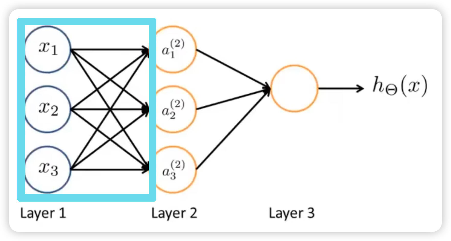
For this image, if we hide the area enclosed by blue-green(cyan) box, we can consider the 2nd layer is the input for the final result. It is using the new feature $a$ instead of the original feature $x$.

XOR and XNOR

XOR: 异或。输入不同值出1，输入相同值出0.

XNOR: 异或非。输入不同值出0，输入相同值出1.

Practical Instances

For sigmoid function, when input is equal to 4.6, the probability is 0.99; vice versa, when input is equal to -4.6, the probability is 0.01

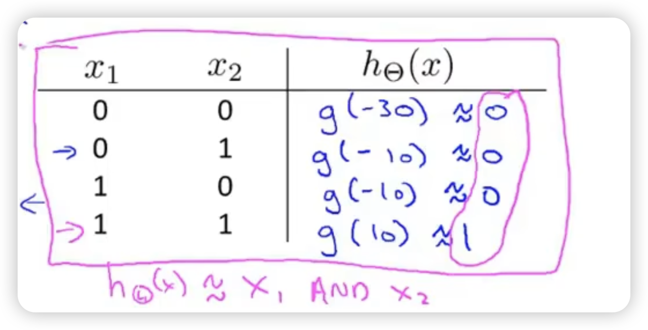
example 1: AND

Only when two inputs are both 1, then output 1. Or output 0/

Two input $x_1, x_2$ and one bias unit $x_0$. $\Theta$: weights function. Every input will have some weight, like coefficient. Then put their linear combination into the input of Sigmoid function.

In this example, we can give weights:

$$\begin{align} \Theta^{(1)}_{10} &= -30\\ \Theta^{(1)}_{11} &= 20\\ \Theta^{(1)}_{12} &= 20\\ \end{align}$$

So we can derive hypothesis, when bias unit $x_0$ is always 1

$$h_\Theta(x) = g(-30 + 20 x_1 + 20 x_2)$$

example 2: OR

Only when two inputs are both 0, then output 0. Or output 1.

The weights are set to -10, 20, 20, deriving $g(-10 + 20x_1 + 20x_2)$

example 3: XNOR

We can put AND, (NOT) AND (NOT), OR together, to compose a network to realize the function of XNOR.

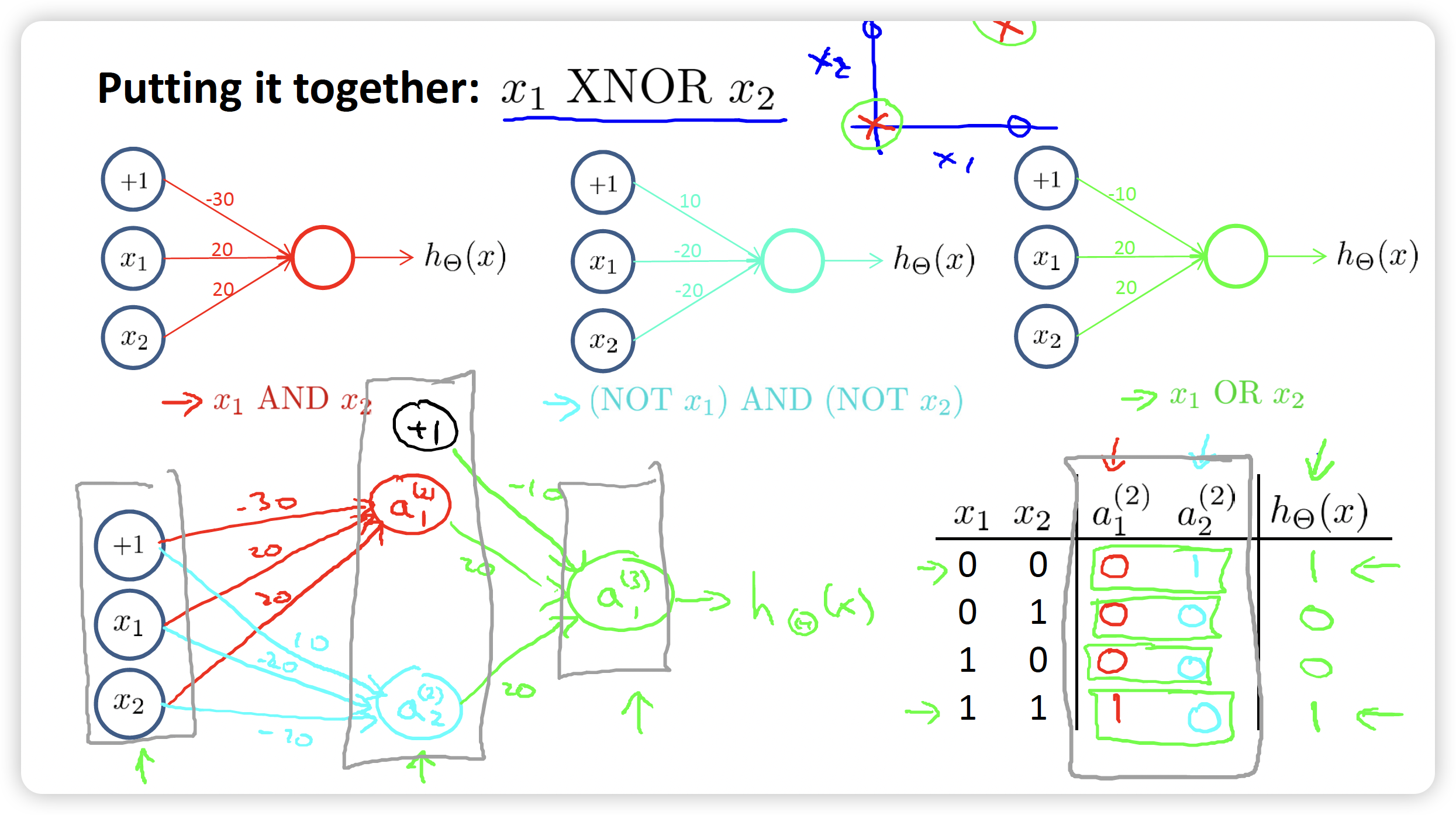
It’s really amazing to implement such a multi layer neural network.

multi variables classification

The output will be changed to four units, namely, a vector. Every unit corresponds to one result. For example, when $h_\theta (x) = [1, 0, 0, 0]^T$, we can know that the first categroy is valid.

If we have only two classes, we just need one output unit to show the result.

If we have more than or equal to 3 classes, we need to use K output units, K is the number of classes.

Cost function

Previously, we learn about Logistic Regression’s cost function:

$$J(\theta) = - \frac {1} {m} \left[\sum_{i=1}^m y^{(i)} \log h_\theta (x^{(i)}) + (1 - y^{(i)})\log (1 - h_\theta (x^{(i)})) \right] + \frac {\lambda} {2m} \sum_{j=1}^n \theta_j^2$$

m is the number of examples we have. n is the number of coefficient. For the last summary, j is from 1 instead of 0 because we don’t include $\theta_0$ due to convention.

When in neural network, there may be several output units and we should calculate them in summary. For the second part, regularization part, we should calculate every element of matrix $\Theta$, so there are 3 sum, respectively for all layers, all rows, all columns, and we exclude the coefficient of $x_0$ in the matrix.

$$J(\Theta) = - \frac {1} {m} \left[\sum_{i=1}^m \sum_{k=1}^K y^{(i)} \log h_\Theta (x^{(i)}) + (1 - y^{(i)})\log (1 - h_\Theta (x^{(i)})) \right] \\ + \frac {\lambda} {2m} \sum_{l=1}^{L-1} \sum_{i=1}^{s_l} \sum_{j=1}^{s_{l+1}} (\Theta_{ji}^{(l)})^2$$

j is the order the row. So, the value of j is the number of the units of next layer l+1.

And when there’s only one output, we don’t need the sum of K, so we have: (the regularization term doesn’t changes)

$$J(\Theta) = - \frac {1} {m} \left[\sum_{i=1}^m y^{(i)} \log h_\Theta (x^{(i)}) + (1 - y^{(i)})\log (1 - h_\Theta (x^{(i)})) \right] \\ + \frac {\lambda} {2m} \sum_{l=1}^{L-1} \sum_{i=1}^{s_l} \sum_{j=1}^{s_{l+1}} (\Theta_{ji}^{(l)})^2$$

forward propagation向前传播

Input the original data to the neural network, and then activate the layer from 1, 2, 3 and so on to the output layer one by one.

back propagation 向后传播

After forward propagation, we have got the output value based on our hypothesis.

Back propagation is to calculate the partial derivative of cost function, namely

$$\frac {\partial} {\partial \Theta_{ij}^{(l)}}J(\Theta)$$

First, calculate the error of the last layer, which is namely the output layer. Error is denoted by $\delta$. Suppose there are 4 layers totally.

$$\delta^{(4)} = a^{(4)} - y$$

Where $a$ is called the prediction of activation unit, $y$ is the real value.

For earlier layer, we have some formula (but I didn’t derive it by myself, just remember and use):

$$\delta^{(3)} = (\Theta^{(3)})^T\delta^{(4)} \cdot g^{\prime}(z^{(3)}) \\ \delta^{(2)} = (\Theta^{(2)})^T\delta^{(3)} \cdot g^{\prime}(z^{(2)})$$

where (from the nature of Sigmoid function):

$$g^{\prime}(z^{(3)}) = a^{(3)} \cdot (1 - a^{(3)}) \\ g^{\prime}(z^{(2)}) = a^{(2)} \cdot (1 - a^{(2)})$$

There’s no error for the 1st layer(input layer)

• Take the case where there is only one sample:

1. Run the forward propagation to get the initial predictive value based on hypothesis.
2. Run the back propagation to get the error of every unit except for the input layer.
3. Calculate partial derivative using the error. (remember below ~)

$$\frac {\partial} {\partial \Theta_{ij}^{(l)}}J(\Theta) = a_j^{(l)} \delta_i^{(l+1)}$$

• Take the case where there is a data set consisting of many samples:

1. Define the matrix $\Delta$ to accumulate the error of every samples.
2. Loop to calculate error for all samples for all units except for the input layer.
3. Add the additive term to the matrix $\Delta$. For one sample, it’s the partial derivative that we can use directly, but for many samples, it’s the additive term to be added up to $\Delta$:

$$a_j^{(l)} \delta_i^{(l+1)}$$

So we update $\Delta$ after calculating every sample:

$$\Delta_{ij}^{(l)} = \Delta_{ij}^{(l)} + a_j^{(l)}\delta_i^{(l+1)}$$

After looping, we can get the partial derivative denoted by $D$:

$$\begin{cases} D_{ij}^{(l)} = \frac 1 m \Delta_{ij}^{(l)} + \frac \lambda m \Theta_{ij}^{(l)}, & \text{if } j \neq 0 \\ D_{ij}^{(l)} = \frac 1 m \Delta_{ij}^{(l)} & \text{if } j = 0 \end{cases}$$

$$D \text { is the partial derivative we want to get} \\ \frac {\partial} {\partial \Theta_{ij}^{(l)}}J(\Theta) = D_{ij}^{(l)}$$

Gradient Checking 梯度检测

To make sure that forward and back propagation is working correctly, especially when using back propagation.

• When $\theta$ is a real number:

We can use the central difference to approximate the gradient.

$$\frac {\rm d} {\rm d \theta} J(\theta) \approx \frac {J(\theta + \varepsilon) - J(\theta - \varepsilon)} {2\varepsilon}$$

Where $\varepsilon$ is usually about 10^-4^

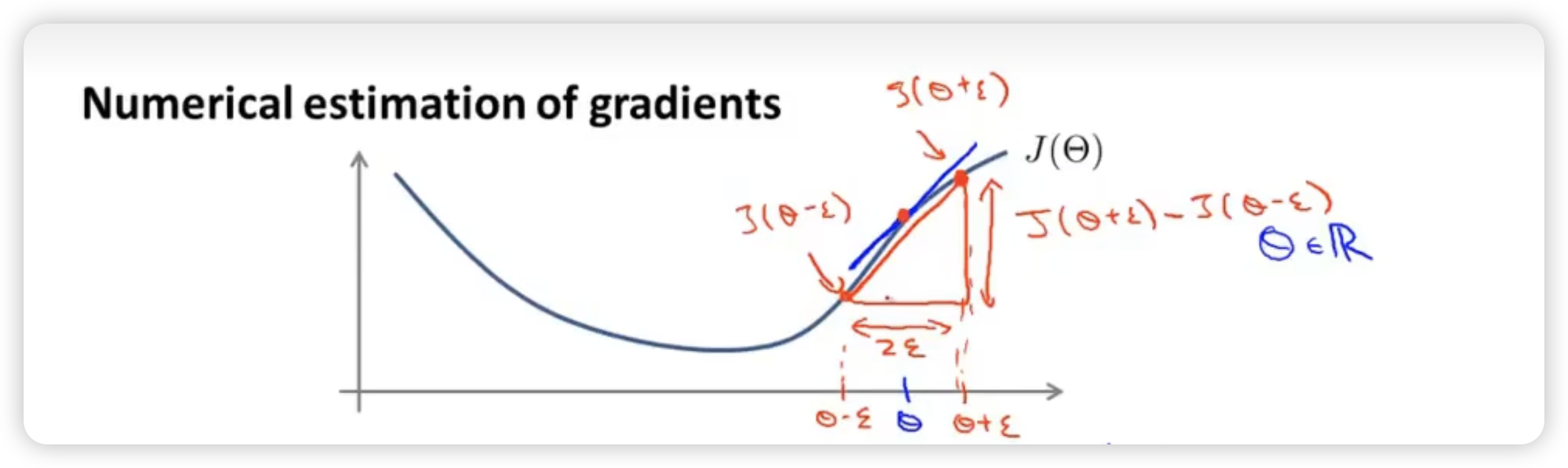
Central difference is more accurate than one-sided difference.

• When matrix or vector*(acutaly the same because we can unroll from matrix to vector)*:

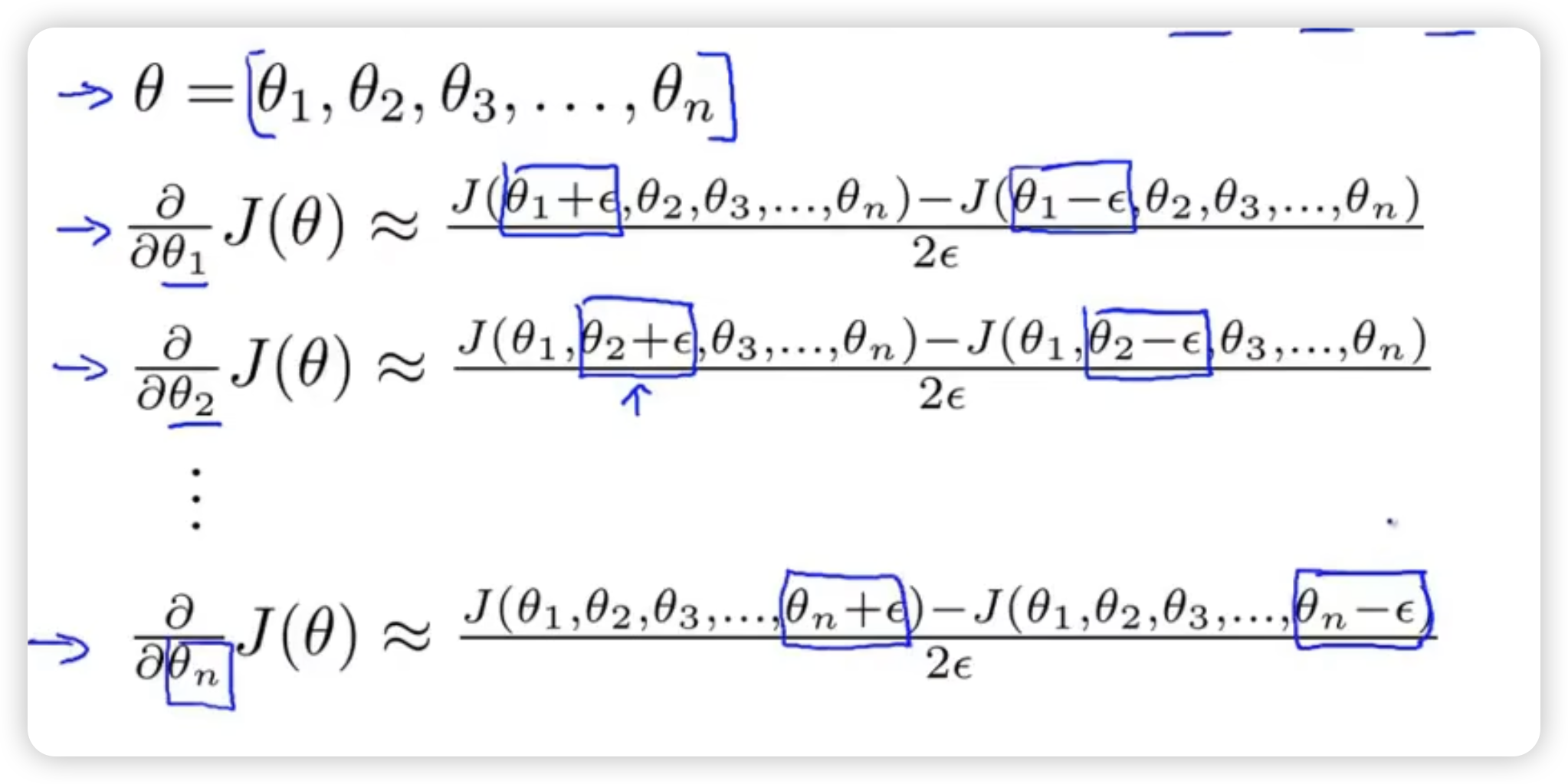
Then check that gradAprrox $\approx$ Dvec from back propagation, to make sure back propagation compute the derivative correctly.

Note:

• When computing the partial derivative, use the back propagation. Numerical gradient is only for checking instead of computing because of its low efficiency.
• Once we verify the implementation of back propagation is correct, disable the gradient checking while we’re training our algorithm.

random initialzation

How can we set the value of initial $\theta$?

• Maybe all-zeros

But the problem is that when we set the same value, the weights will be always the same without any difference. It’s not friendly for us to let neural network learn more interesting functions. This is called symmetric weights

• Random Initialization

This method is to break the situation of symmetry. Generate random value for every $\theta$ between $-\epsilon$ and $\epsilon$.

put it together

To train a neural network, the first step is to pick a network architecture (connectivity pattern连接模式 between neurons): how many layers, how many units per layer

Number of the input units: Dimension of features $x$

Number of the output units: Number of classes类别的数量

Reasonable default: 1 hidden layer. If more than 1 hidden layer, every hidden layer have the same number of units. (usually the more the better)

For example, if we have 10 classes, then our output will be a 10-dimensional vector which has 1 in the valid position and 0 in other positions.

training a neural network

1. Randomly initialize weights

2. Implement forward propagation to get $h_{\theta}(x^{(i)})$ for any $x^{(i)}$

3. Implement code to compute cost function $J(\Theta)$

4. Implement back propagation to compute partial derivative.

5. Gradient checking. Then disable it.

6. Use gradient descent to minimize cost function.